Landscape classification and karst management at Jenolan Caves, NSW
INTRODUCTION
Karst is a complex and highly variable landscape, operating within a variety of scales. Landscape classification is a tool that allows managers to deal with this complexity, by defining land units at various scales, to which differing management strategies can be applied. The challenge in developing a landscape classification model for karst is to identify that appropriate scale which accounts for the most meaningful detail, while still being achievable in terms of field survey and data handling. This is the SLAP principle - Simplify as Little As Possible. At the same time, the model must simplify the details enough to make meaningful statements about the nature of the landscape.
WHAT IS LANDSCAPE CLASSIFICATION?
Landscape classification is essentially a mapping technique, and has been in use in Australia since at least the 1950s. Patterns in the landscape are defined by a hierarchical process involving the identification of land classes. Each class level is identified at a particular scale, e.g.
large scale (> 10 000 ha) > medium scale > small scale (< 1 ha)
At the smallest scale, land classes are distinctive, homogenous (uniform) environments (e.g. gently sloping red earth plain on limestone with Eucalyptus woodland). At the largest scale, the land classes are heterogeneous (varied), but are broadly linked by an underlying similarity (e.g. Southern Highlands of Eastern Australia).
Landscape classification helps to make sense of complex environments by providing uncomplicated information in the form of maps. Supporting documentation may include tables defining the characteristic features of a class. With few exceptions (e.g. Godwin 1991), the technique has not been specifically applied to karst. However, there is wide range of potential applications for karst managers.
APPLICATIONS OF LANDSCAPE CLASSIFICATION
Landscape classification can provide a framework for a variety of applications including:
- Land capability assessment
- Risk assessment and monitoring
- Gap analysis
- Threatened species habitat identification and assessment
- Integrated catchment management
- Identifying links between surface and underground environments
The framework afforded by landscape classification provides a spatial context for understanding the environmental relationships of particular areas. At smaller scales, the distribution of related areas can be identified, so it is then possible to determine for example, the distribution and extent of landscapes that are susceptible to accelerated erosion. Such information is useful in assessing the type of land use suitable for an area, and assists in identifying sites which need to be prioritised for risk assessment and monitoring.
As another example, site records for rare and threatened species can be incorporated into the classification. Patterns of distribution of sites within land classes can be determined, and predictions of the locations of populations outside of known distribution areas can be determined. This provides a basis for gap analysis. Under-representation of a rare and threatened species habitat within the reserve boundaries, or gaps in management knowledge can be identified. This may provide a basis for requisition policies and recovery plans (in the case of under-representation) or a focus for surveys and monitoring programs.
These types of applications apply to any landscape, but there is one application that may prove particularly useful to karst. By linking cave maps to land class maps (e.g. by using overlays in GIS models), it may be possible to provide useful information about interrelationships between the surface and subterranean environments. For example, if a cave system is largely located within a single land class, energy inputs into the cave can be predicted, which will have implications for managing cave fauna. In addition, previously unknown hydrological links between surface and subsurface flows may be detected by this application of landscape classification.
BENEFITS OF LANDSCAPE CLASSIFICATION
Aside from a wide range of applications, landscape classification has many benefits for the karst manager.
- It provides a means by which to make sense of complex environments.
Natural environments are by nature heterogeneous, and it is often difficult to identify interrelationships within a landscape without an understanding of the component parts of the landscape, and how those component parts are distributed. - It provides a rational and cohesive framework for collecting
and analysing environmental data.
The landscape classification provides a means of partitioning environmental data in a logical, step-wise manner. It also provides a spatial context for understanding the dynamics of a particular site, species, landform or ecosystem at various scales. - It provides a biophysical basis for assessing resources.
Natural landscapes operate independently of political and cadastral boundaries. Landscape classification provides a more meaningful ecological basis for understanding the environment. - It allows the adoption of a uniform management approach.
At the finer scales of the classification hierarchy, the distribution of land classes becomes increasingly patchy. By using a landscape classification map, related areas separated by some distance can be identified, and uniform management policies can be applied. - It allows for rapid and cost-effective assessments.
Having identified a group of homogenous land classes, verification of the mapping predictions only requires limited field assessment of a representative set of sites. This reduces the time spent in the field and the costs of the field survey.
LANDSCAPE CLASSIFICATION HIERARCHY FOR JENOLAN CAVES
Class Definition
Classes are typically defined according to a set of characteristic attributes, including:
- climate
- geology, geomorphology
- soils
- vegetation
- hydrological regime
At each scale of the landscape classification hierarchy, the level of detail in the class descriptions changes accordingly. Hence large-scale classes require very broad descriptions, and small-scale classes are highly detailed. For Jenolan Caves four class levels have been determined as shown in Figure One. These are:
Bioregion (>1:250 000) > Land Province > Land System > Land Unit (< 1:10 000)
To date, efforts at Jenolan have concentrated on defining Land Unit boundaries. As the Jenolan mapping project is using a bottom-up approach to classification, intermediate land class boundaries will result from the amalgamation of these fine-scale land units.
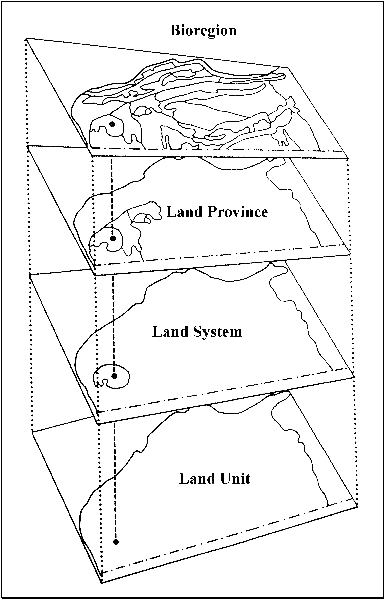
Figure 1: Landscape Classification hierarchy as applied to Jenolan Karst Conservation Reserve.
Bioregions
The Bioregion is the broadest delineation of the land classes applied to Jenolan, and is mapped at scales greater than 1: 250,000. Uniform geology, climate, landforms and broad vegetation types define boundaries for units within this class. A Bioregion boundary has already been determined by external agencies for Jenolan Caves. Jenolan is encompassed by the South Eastern Highlands Bioregion, the boundaries of which occur outside of the reserve. The Bioregion is described as:
Steep dissected and rugged ranges extending across southern and eastern Victoria and southern NSW. Geology predominantly Paleozoic rocks and Mesozoic rocks. Vegetation predominantly wet and dry sclerophyll forests, woodland, minor cool temperate rainforest and minor grassland and herbaceous communities.(Thackway 1996).
Knowledge of the attributes of the Bioregion provides a regional context for understanding the characteristics of Jenolan Caves, and the external processes influencing the reserve.
Land Provinces
Land Provinces are mapped at broad to intermediate scales (1: 100 000 to 1:250 000). They are delimited by a finer scale separation of geology and landform characteristics than those identified for a Bioregion. In addition, information about broad soil and vegetation patterns is also incorporated. As an example, a Bioregion dominated by igneous rocks with (1) high altitude inland ranges with rainforest on shallow soils, (2) a coastal plain blanketed by alluvials with open sclerophyll woodlands and (3) medium altitude coastal ranges with sandy soils and vine forests, would be divided into three provinces.
Land Systems
Land Systems are mapped at intermediate scales varying between 1:10 000 to 1: 100 000. The separation of Land Systems is on the basis of fairly uniform geological and landform elements with related suites of soils and vegetation patterns found within a provincial boundary. For example, if the coastal plain (described above as Province 2) contained (a) transitional foothills, ranges and isolated peaks of igneous rock with clay loams and closed forest; (b) coastal alluvial plains on an igneous base with sandy soils and open forests and woodlands and (c) subtidal/intertidal lowlands with sandy clays and mangrove, saltmarsh and aquatic plant communities, then three land systems would be described.
Land Units: The Minimum Mapping Unit (MMU)
It was earlier stated that the challenge in developing a landscape classification model for karst is to identify that appropriate scale which accounts for the most meaningful detail, while still being achievable in terms of field survey and data handling. The minimum mapping unit is the smallest object that must be mapped within the hierarchy. For Jenolan Caves Reserve, this has been identified as the Land Unit. The Land Unit is mapped at scales of 1:10 000 or less.
A Land Unit is defined as a homogeneous area of terrain and vegetation which is clearly identifiable, and which has ecological significance (Figure 2). Class boundaries are defined primarily on uniform topography with a distinctive soil and water regime and plant community. From the example of the previous section, a Land Unit might be the mangrove communities of Land System 3. An example from Jenolan Caves Reserve is the Limestone Ledge Land Unit. This is identified by the presence of steep cliffs and bluffs in limestone, with shallow stony soils and a Bursaria low shrubland, and is an important habitat for Brush-Tailed Rock Wallabies. Further guidelines for developing a landscape classification are provided in Appendix One.
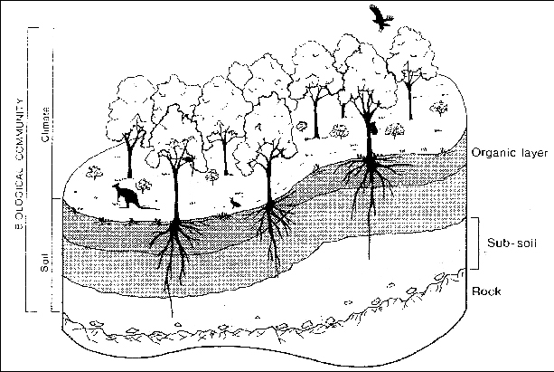
Figure 2: Example of a land unit, the minimum mapping unit for landscape classification at Jenolan. Specific plant and animal community information is incorporated at this scale.
SCALE-DEPENDENT LIMITATIONS OF LANDSCAPE CLASSIFICATION
The determination of the MMU for any landscape classification is critical. This will allow managers to determine if commercially available data is adequate for their purposes, or whether customised data needs to be obtained. Most State government agencies will provide data at the Land Province scale i.e. 1:100 000 to 1:250 000. While this may be adequate for regional studies, the generalisations inherent in such data may make them inappropriate or inaccurate for analysis at the Reserve scale. Thus the successful mapping of a reserve probably requires customised data, for which managers need to determine a minimal mapping unit (MMU) which provides meaningful data while still being achievable in terms of time and cost.
The minimal mapping unit is the smallest object that must be mapped in a hierarchy. A rule of thumb is that the MMU is four times the resolution of the data needed. Thus if you want to map spatial objects that are 20m by 20m (0.04ha), then the data you use must have a resolution of 5m by 5m. From this it is apparent that on an aerial photograph with a resolution of 0.5m you can map to ~5m2 while if you are using a Landsat TM satellite image (resolution 25m), you can map down to about 1ha (100 by 100m). This may be adequate for a whole Reserve, but will fail to detect small land units such as individual vegetated limestone ledges.
There are a large number of image products available for mapping (Table 1), with the newest possessing both high spatial resolution and ability to sense beyond the visible light wavelengths. In particular, the use of near infra-red light (NIR) allows calculation of various indices of vegetation health, which have wide applications in forest inventory, weed detection, and survey of algal blooms.
| Data Source | Spatial resolution | Spectral resolution | Repeat cover | MMU |
| Landsat TM | 25m | 7 bands - B G R NIR NTIR 2xTIR | 16 days | 1ha |
| Spot XS | 20m | 3 bands - BG R NIR | 26 days; +5 off-nadir | 0.6ha |
| SpotPan | 10m | 1 band - invisible BG to R | 26 days; +5 off-nadir | 0.2ha |
| CSU Airborne Video System | 1m | 4 bands - B G R NIR | On demand | 20m2 |
| Digital Colour Air Photos | 0.5m | natural colour or false infrared | On demand | 5m2 |
Table 1: Readily available sources of digital image data and their characteristics.
USES AND ABUSES OF DEMS
One of the most useful items of data that can be obtained is a digital elevation model (DEM). DEMs are the building blocks of topographic maps, as well as much else. The original data are spot heights from aerial photography, on an irregular grid. From these, a triangular interpolation network can be built to account for variations in terrain complexity. Areas of low relief are next masked out to avoid spurious pits and pinnacles. For Jenolan, the final surface was interpolated using a cubic spline technique to give a 5m horizontal resolution cellular DEM (Figure 3) with data range from 663 to 1233m.
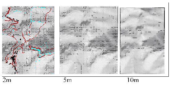
Figure 3: Comparison of DEMs with differing spatial resolution, Jenolan Caves Reserve
From DEMs the following products can be derived:
- Contours at any desired interval
- 3-D terrain models
- Topographic profiles
- Slope maps
- Aspect maps
- Maps of specified altitude ranges
These can be used to display other data or as input layers to a GIS. Commercially available DEMs (such as those supplied by AUSLIG or the State mapping agencies) are usually derived from existing topographic maps or stereo satellite images. They have a large cell size (typically 25m) and from them one can generate 20m contours at best. But this resolution may be inappropriate for detailed work, as the MMU from these will be 1ha.
Determining the appropriate cell size for a DEM relies on spatial analysis of the terrain and some knowledge of the limitations of the initial data set. One technique that is widely used is that of spatial autocorrelation (Worboys, 1995). This rather weighty word relies on the assumption that the elevation within a single cell will rely to a greater or lesser degree on the adjoining cells. We would normally expect that in a normal landscape the value of a point elevation on a slope would relate closely to those above and below it. That is, there is significant spatial correlation in the landscape. In karst terrain, as we know, this assumption is not always valid because of the presence of dolines, pinnacles and cliffs that create local anomalies in elevation.
We measure this using a statistic called Moran's I, which measures the statistical relationship between each cell and those surrounding it, over successively larger distances. From it we can estimate the distance at which Moran's I significantly reduces in value. This can be used to estimate an MMU and thus the resolution of the data we need to adequately account for the local variability in the karst terrain. In Figure 4, this has been carried out for the Jenolan DEM. The graph defines a MMU at 20m, implying that we need a data resolution of 5m. This is unavailable from State data, but by using digital aerial photography at a scale of 1:12,500 we can achieve it.
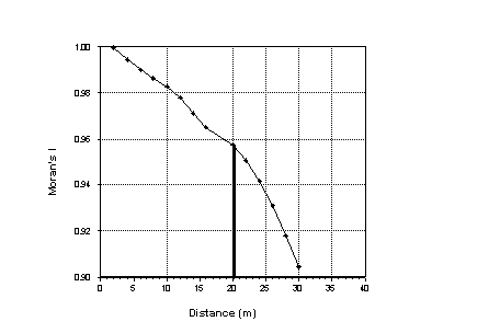
Figure 4: Results of Moran's I analysis for Jenolan DEM
Once we have our DEM, we can classify it according to slope angle to identify flat spots that correspond to limestone ledges. Or we can use it to produce a map that shows areas visible or invisible from a given point or line on the terrain (the military notion of live and dead ground). This viewshed can be used to assess the visual impact of new buildings, carparks or even aerial cablecars. We can combine it with other data on vegetation type to predict where rare plants of known preference might occur. The applications are limited only by our imagination.
CONCLUSIONS
Land classification provides a means of understanding landscape patterns and processes and can be of value to managers in providing a transparent and objective framework for management actions. Land classification rests on a hierarchy of mapping units from land province to land unit. For most karst systems, the land unit will be the appropriate mapping scale and for this data will need to be at a scale around 1;10 000. For many reserves one may need customised data rather than the generic data that are available through State agencies. Digital elevation modelling provides a highly valuable product which can be translated into other forms such as slope, aspect etc. Careful attention needs to be paid to the resolution of the DEM so that the complexity of karst terrain is faithfully rendered.
BIBLIOGRAPHY
Godwin, M. 1991. Land Units of the Chillagoe Area - Queensland. Chillagoe Caving Club / Queensland National Parks and Wildlife Service. Cairns.
Gunn, R.H., Beattie, J.A., Riddler, A.M.H and Lawrie, R.A 1988. Mapping. In R.H. Gunn, J.A. Beattie, R.E. Reid and R.H.M van de Graaff (eds).Guidelines for Conducting Surveys. Australian Soil and Land Survey Handbook, Volume 2. Inkata Press. Melbourne. pp. 90-112.
Thackway, R. 1996. The Interim Biogeographic Regionalisation of
Australia
http://www.biodiversity.environment.gov.au/environm/wetlands/bioreg.htm
Worboys, M.F. 1995. GIS - a Computing Perspective, Taylor & Francis, London, 376pp.
APPENDIX ONE: GUIDELINES FOR MAPPING
Prior to commencing a landscape classification mapping project it is vitally important to determine:
- the applications of the final landscape classification for your situation;
- the benefits you expect from your landscape classification, and;
- the minimum mapping unit (MMU) that will satisfy your needs and expectations.
The following guidelines provide a good basis for planning landscape classification mapping:
- Collect and collate all available information of land attributes (geology, soils, vegetation). This may be available in the form of published maps, reports, databases, etc.
- Acquire the best available field mapping topographic base. Normally satellite imagery, airbourne video and/or aerial photography. May need to be customised if commercially available data is not at an appropriate scale.
- Conduct a brief field survey to identify likely land units and land systems matching imagery with ground truthing. A familiarisation process that will allow better interpretation of the available imagery. Allows the assessment of areas that are obscured on the imagery.
- Conduct an interpretation of available imagery to create a preliminary landscape classification. The first stage of mapping, where the number of land classes and their distribution and boundaries are provisionally determined.
- Conduct field mapping and survey to refine class boundaries, and acquire ecological data. Carry out routine mapping, confirming land class boundaries and modifying them as required.
- Construct GIS data layers or hard copy maps. The final landscape classification map can now become the basis for management of the reserves.
Modified from Gunn et al (1988)
Generally, the MMU that can be shown on a map is the Land Unit. While Land Units are essentially homogenous, minor variations may be present that may have ecological significance. The best approach for recording such variations is to provide a series of profile diagrams. For the Limestone Ledge Land Unit, the profile diagrams may show the variations in ledge shape, slope and height as illustrated in Figure 5. Profile diagrams are not included on the land classification map, but can be appended to the map as tables.
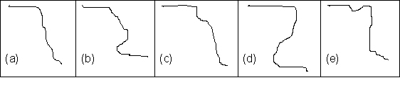
Figure 5: Examples of hypothetical profile diagrams for Limestone Ledge Land Unit, Jenolan Caves Reserve.